(Click on image to see enlargement)
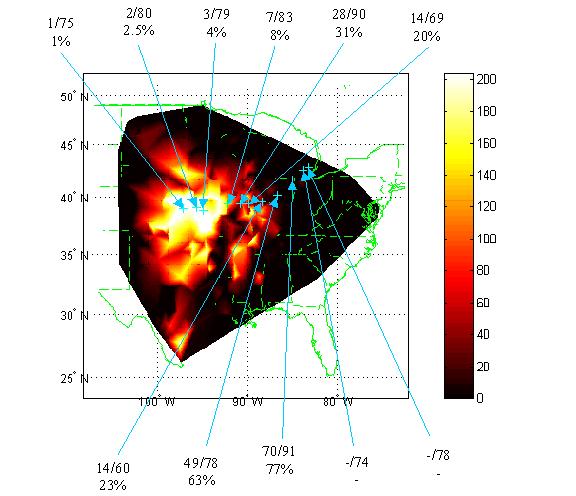
A plot of variation in abundance of the Dickcissel (Spiza Americana, in the Cardinal family)
over its species range. At 11 selected points, each successively further from the peak abundance,
the pullouts show the ranks of the species in terms of local abundance within the community
(1 is highest) relative to total number of species in the community and the percentile of abundance
within the community (to adjust for communities that differ in number of species). A "-" indicates that
the species is absent from that community even though it is within the range. Note that as we get further
from the peak the abundance drops off, and in particular drops off quite quickly from the peak and then has
a long tail of low abundance.
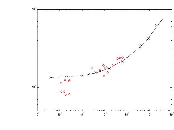
(Click on image to see enlargement) This graph shows the simulated SPAR model (X symbols with line showing an average across 10 Monte Carlo simulations) vs. Preston's (1960) data for birds of North America (O symbols). The line is nearly horizontal between the leftmost two points as described in the text. Note that in this same region the data for scales smaller than 104 km2 falls below the line. This is because SPARs at small scales are driven by sampling effects and habitat heterogeneity, which are not included in our model. The rest of the line is a fit of an exponential curve in log-log space. Except at the very small scales, we can see that the simulated data comes extremely close to the observed data, especially given that no fitting parameters were used. The simulation correctly predicts the c-value (intercept), z-value (slope) and region and degree of curvilinearity.
This graph is unique because it has no parameters derived from the data to which the curve is fit. All parameters
are derived a priori
(Click on image to see enlargement)
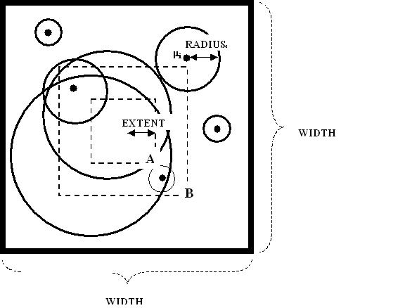
A pictorial representation of the SPAR simulation model and its parameters. A continent of dimensions
WIDTH x WIDTH is created. Within this continent, the centers, mi, of species are placed down randomly
using a Poisson process. For each center a RADIUS is randomly sampled. One alternative for the distributions
of the radii is to resample from an empirical distribution of range sizes. Another alternative is to use
equation (2) and specify distributions for NMAXi, si and the value of NMIN. See the text for descriptions of
the distribution of radii. Ranges are treated as circular. A progressively larger series of boxes is drawn,
each with a size of EXTENT x EXTENT where the maximum EXTENT=WIDTH/2. In the above figure, BOX A has a species
diversity of 3 (inside of two range and intersects a 3rd). BOX B has a species diversity of 5
(the previous 3, one whose range is completely included and one whose range it intersects).
The total diversity of the continent, S, is 7. S is an input parameter to the model.
Brian McGill's home page